Tutorial
The first step in fitting a model to an observed spectrum is to read the
spectrum into the appropriate format. See Data format for an explanation
of the format and an example, and Units system for a brief explanation of the
unit system used in Naima. We load the spectral data with
astropy.io.ascii:
from astropy.io import ascii

data = ascii.read("RXJ1713_HESS_2007.dat")
Building the model and prior functions
The model function is the function that will be called to compare with the observed spectrum. It must take two parameters: an array of the free parameters of the model, and the data table.
Naima includes several models in the naima.models module that make it
easier to fit common functional forms for spectra (PowerLaw,
ExponentialCutoffPowerLaw, BrokenPowerLaw, and
LogParabola), as well as several radiative models
(InverseCompton, Synchrotron,
Bremsstrahlung, and PionDecay; see
Radiative Models for a detailed explanation of these). Once initialized with the
relevant parameters, all model instances can be called with an energy array to
obtain the flux of the model at the values of the energy array. If they are
called with a data table as argument, the energy values from the energy
column will be used.
Building the model function from one of the radiative models is easy. In the
following example, the three model parameters in the pars array are the
amplitude, the spectral index, and the logarith or the cutoff energy. We first
add the necessary units for the radiative model and then compute and return the
model flux for the energies contained in the data table:
from naima.models import ExponentialCutoffPowerLaw, InverseCompton
import astropy.units as u


def model(pars, data):
    amplitude = pars[0] / u.eV
    alpha = pars[1]
    e_cutoff = (10 ** pars[2]) * u.TeV

    ECPL = ExponentialCutoffPowerLaw(amplitude, 10 * u.TeV, alpha, e_cutoff)
    IC = InverseCompton(
        ECPL,
        seed_photon_fields=[
            "CMB",
            ["FIR", 26.5 * u.K, 0.415 * u.eV / u.cm ** 3],
        ],
    )

    return IC.flux(data, distance=1.0 * u.kpc)
In addition, we must build a function to return the prior function, i.e., a
function that encodes any previous knowledge you have about the parameters, such
as previous measurements or physically acceptable ranges. Two simple priors
functions are included with Naima: normal_prior, and
uniform_prior, and loguniform_prior. uniform_prior
can be used to set parameter limits. Following the example above, we might want
to limit the amplitude to be positive, and the spectral index to be between -1
and 5:
from naima import uniform_prior


def lnprior(pars):
    lnprior = uniform_prior(pars[0], 0.0, np.inf) + uniform_prior(pars[1], -1, 5)
    return lnprior
Selecting a starting point for the sampling
Before starting the MCMC run, we must provide the procedure with initial estimates of the parameters and their names:
p0 = np.array((1e33, 3.0, np.log10(30)))
labels = ["norm", "index", "log10(cutoff)"]
This example is relatively simple, but for more complicated models (in particular those with more than one emission channel, such as Synchrotron and Inverse Compton) it may be difficult to provide an adequate initial parameter vector without comparing it visually with the spectra. For these models, an initial parameter vector far from the maximum likelihood vector may mean that during the minimization or sampling process the algorithm gets stuck in a local maximum.
In order to make an adequate estimation easier, Naima provides a tool to
interactively see the output of the model and compare it with the observed data
while changing the parameter values. This tool can be accessed in two ways: the
first is setting interactive=True in the options of get_sampler or
run_sampler (see below in sampling for details on these functions).
This will launch an interactive matplotlib window in which the parameters can
be changed and the resulting model compared to the observed spectra. With each
change, the log probability of the model given the observed spectra is computed.
In addition, a Nelder-Mead fit can be launched from a button in the window to
find the maximum likelihood parameter vector. Once you are happy that the
current model is a good approximation to the observed spectrum, closing the
window (whether through the window manager or the Close window button) will
use the current parameter vector as a starting point for the sampling procedure.
The alternative way of accessing the interactive fitter is to access it directly
through the class naima.InteractiveModelFitter from an interactive Python
interpreter.
The parameter vector shown in the interactive window can be accessed through the
imf.pars attribute, and then copied to a new p0 variable to be used in
the sampling:
>> imf = InteractiveModelFitter(model, p0, data=data, labels=labels)
>> # interactive fitting done
>> p0 = imf.pars
Note that the data argument can be omitted and an energy range specified through the
e_range argument to inspect the behaviour of the model independently of the
data:
>> imf = InteractiveModelFitter(model, p0, e_range=[1 * u.GeV, 100 * u.TeV])
Sampling the posterior distribution function
All the objects above can then be provided to run_sampler, the main
fitting function in Naima:
sampler, pos = naima.run_sampler(
    data_table=data,
    p0=p0,
    label=labels,
    model=model_function,
    prior=lnprior,
    nwalkers=128,
    nburn=50,
    nrun=10,
    threads=4,
)
The nwalkers parameter specifies how many walkers will be used in the
sampling procedure, nburn specifies how many steps to be run as burn-in,
and nrun specifies how many steps to run after the burn-in and save these
samples in the sampler object. For details on these parameters, see the
documentation of the emcee package.
Inspecting and analysing results of the run
The results stored in the sampler object can be analysed through the plotting
procedures of Naima: plot_chain, plot_fit, and
plot_data. In addition, two convenience functions can be used to
generate a collection of plots that illustrate the results and the stability of
the fitting procedure. These are save_diagnostic_plots and
save_results_table:
naima.save_diagnostic_plots(
"RXJ1713_IC",
sampler,
blob_labels=[
"Spectrum",
"Electron energy distribution",
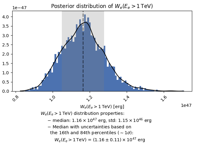
"$W_e (E_e>1$ TeV)",
],
)
naima.save_results_table("RXJ1713_naima_fit", sampler)
The saved table will include information in the metadata about the run such as
the number of walkers n_walkers and steps n_run sampled, the initial
parameter vectori p0, the parameter vector with the maximum likelihood
ML_pars and the maximum value of the negative log-likelihood
MaxLogLikelihood. The table itself shows the median and upper and lower
uncertainties (50th, 84th, and 16th percentiles of the posterior distribution)
for the parameters sampled:
n_walkers         : 128
n_run             : 100
p0                : [1.3884430349732936e+32, 2.5717536865466712, 1.6821145924203185]
ML_pars           : [1.3697204402514948e+32, 2.5839150825284958, 1.7002798209378214]
MaxLogLikelihood  : -17.98655803890747

------------- ------- ------- --------
        label   median   unc_lo  unc_hi
------------- -------- -------- -------
         norm 1.38e+32 8.57e+30 1.1e+31
        index     2.57    0.115   0.103
log10(cutoff)     1.69    0.109   0.115
       cutoff     48.9     10.9    14.8
The table is saved by default in ECSV format which can be
easily accesed with the astropy.io.ascii module.
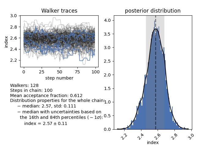
Plotting functions: chains
The function plot_chain will show information about the MCMC chain for
a given parameter. It shows the parameter value with respect to the step number
of the chain, which can be used to assess the stability of the chain, a plot of
the posterior distribution, and several statistics of the posterior
distribution. One of these is the median and 16th and 84th percentiles of the
distribution, which can be reported as the inferred marginalised value of the
parameter and associated \(1\sigma\) uncertainty. For the electron index
(parameter 1), plot_chain shows:
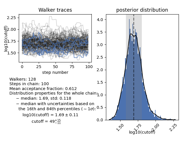
For parameters that have been sampled in logarithmic space and their parameter
label includes log10 or log, plot_chain will also compute the
value and percentiles in linear space:
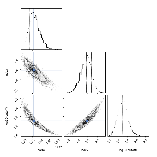
The relationship between the samples of the different parameters can be seen
though a corner plot with
plot_corner which is a wrapper around corner.corner. The maximum
likelihood parameter vector can be indicated with cross:
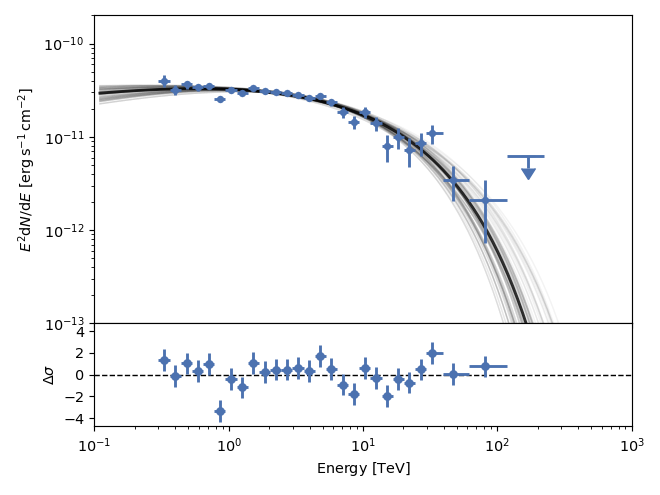
Plotting functions: fit
The plot function plot_fit allows for several ways to represent the
results of the MCMC fitting. By default, it will show the Maximum Likelihood
model with a black line, and 100 samples from the posterior distribution in
gray:
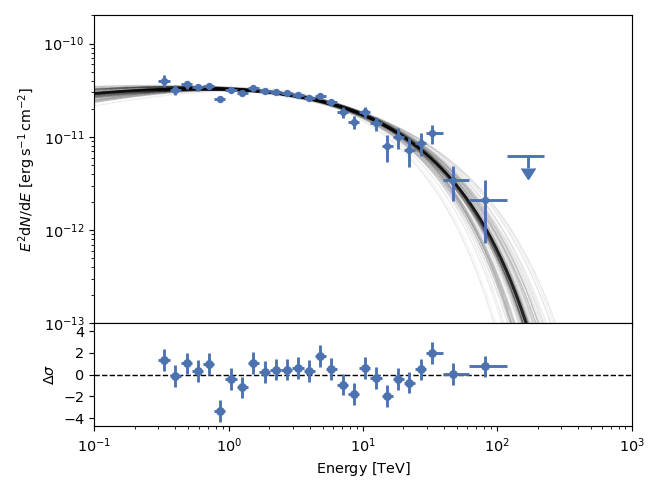
The 100 samples are taken from the blobs stored in the sampler, so they only
contain the model values at the observed flux points. If you want to show the
samples and ML model for a wider energy range (or between energy bands like
X-ray and gamma-ray) you can use the e_range parameter. Note that the model
will be recomputed n_samples times (by default 100) when plot_fit is
called, so this may significantly slow the plot speed if the model function
calls are expensive. Setting e_range=[100*u.GeV, 100*u.TeV], we obtain the
following plot:
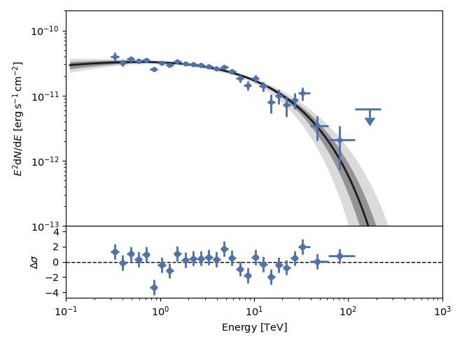
The spread of the parameters in the posterior distribution can also be
visualized as confidence bands. Using the confs parameter of plot_fit, a
confidence band will be computed for each of the confidence levels (in sigma)
given in confs. Setting confs=[3,1], the confidence bands at
\(1\sigma\) and \(3\sigma\) are plotted. Note that no samples are shown
if the confs parameter is set:
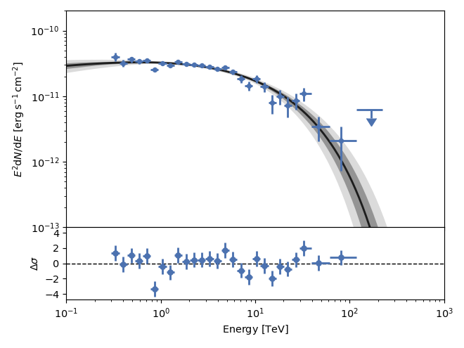
As for the plot showing the samples, the energy range for the confidence bands
can be set through the e_range parameter. The number of samples needed will
be computed so that the highest confidence level given can be constrained. This
results in 740 samples for a \(3\sigma\) confidence level:
Saving and retrieving the results of the sampling run
The parameter chain and metadata blobs resulting from the sampling procedure can
be saved with naima.save_run. This function will save the results of the run
to an HDF5 file that can be archived and analysed after the fact. The sampler
properties saved to the HDF5 file are:
parameter vector chain:
sampler.get_chain()log-probability for all the parameter vectors in the chain:
sampler.get_log_prob()metadata blobs:
sampler.get_blobs()parameter labels:
sampler.labelsdata table:
sampler.data
Note that only metadata blobs that can be converted into a numpy array will be
stored. Blobs consisting of other classes, or with different lengths within the
same blob, will raise a warning and may be discarded on the naima.save_run call.
The saved sampler can be retrieved with the naima.read_run function, which
will return an EnsembleSampler-like object. However, the model function
cannot be saved in the HDF5 file, so a model function has to be provided at read
time. This function will be used to compute the model output from the parameter
vectors in the chain. Without a model function, the sampler read from the HDF5
file can be passed onto plot_chain, plot_corner,
plot_fit, and plot_data for analysis. If a model function is
provided to naima.read_run, the resulting sampler can also be used with
plot_fit when setting the e_range parameter, which requires the
model function to be accesible in the modelfn attribute of the sampler
object provided.
Saving additional information — Metadata blobs
If we wish to save additional information at each of the model computations, extra information can be returned from the model call. This extra information (known as metadata blobs; see details in the emcee documentation) is stored in the sampler object returned from the fitting procedure and can be accessed later. There are three formats for the data stored as a metadata blob that will be understood by the plotting routines of Naima:
A
Quantityscalar. A histogram and distribution properties (median, 16th and 84th percentiles, etc.) will be plotted.A
Quantityarray with the same length as the observed spectrum energy array. If it has a physical type of flux or luminosity, it will be interpreted as a photon spectrum and plotted against the observed spectrum energy array.A pair (tuple or list) of
Quantityarrays of equal length. They will be plotted against each other.
When fitting a radiative output to a spectrum, information on the particle distribution (e.g., the actual particle distribution, or the total energy in relativistic particles) can be saved as a metadata blob. Below is an example that does precisely this with an Inverse Compton emission model:
from naima.models import ExponentialCutoffPowerLaw, InverseCompton
import astropy.units as u
import numpy as np


def model_function(pars, data):
    amplitude = pars[0] * (1 / u.eV)
    alpha = pars[1]
    e_cutoff = (10 ** pars[2]) * u.TeV
    e_0 = 10 * u.TeV

    ECPL = ExponentialCutoffPowerLaw(amplitude, e_0, alpha, e_cutoff)
    IC = InverseCompton(
        ECPL,
        seed_photon_fields=[
            "CMB",
            ["FIR", 26.5 * u.K, 0.415 * u.eV / u.cm ** 3],
        ],
    )

    # The total enegy in electrons of model IC can be accessed through the
    # attribute We or obtained for a given range with compute_We
    We = IC.compute_We(Eemin=1 * u.TeV)

    # We can also save the particle distribution between 100 MeV and 100 TeV
    electron_e = np.logspace(11, 15, 100) * u.eV
    electron_dist = ECPL(electron_e)

    # The first object returned must be the model photon spectrum, and
    # subsequent objects will be stored as metadata blobs
    return IC(data), (electron_e, electron_dist), We
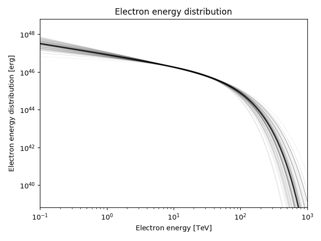
The additional quantities we have stored can the be accesed via the
sampler.get_blobs method. The function plot_blob allows to plot them
and extract distribution properties. For the blobs that are a tuple or have the
same length as data['energy'], they will be plotted as spectra:
and for the ones that are a scalar value, such as the total energy in electrons that we returned as the third object, a histogram and distribution properties will be plotted: