Radiative Models

Naima contains several radiative models that can be used to compute the non-thermal emission from populations of relativistic electrons or protons. Below there is a brief explanation of each model, and full details on the physics and motivation for the implementation can be found in the referenced articles.

All the radiative models take a particle distribution function as a first argument. Several particle distribution functions can be found in the naima.models module: PowerLaw, ExponentialCutoffPowerLaw, LogParabola, BrokenPowerLaw, and ExponentialCutoffBrokenPowerLaw. To use them as a particle distribution function the units of their amplitude must be in particles per unit energy (i.e., convertible to 1/eV). If you have computed a particle distribution from a physical code and wish to compute its radiative output, you can use the TableModel class to define a distribution function from an array of energies and an array of particle numbers per unit energy.

Here is an example of how you can use the Exponential Cutoff Power Law model as particle distribution function for an inverse Compton model (see below in IC for details about the inverse Compton model).

>>> ECPL = naima.models.ExponentialCutoffPowerLaw(
...     1e36 * u.Unit("1/eV"), 1 * u.TeV, 2.1, 13 * u.TeV
... )
>>> IC = naima.models.InverseCompton(ECPL, seed_photon_fields=["CMB"])

The parameters of the particle distribution can be accessed through the particle_distribution attribute of the radiative model, e.g.:

>>> IC.particle_distribution.index = 1.8
>>> print(ECPL.index)
1.8

In addition, the same particle distribution instance can be used for several radiative models simultaneously, for example when computing the synchrotron and IC emission from an electron population:

>>> SYN = naima.models.Synchrotron(ECPL, B=100 * u.uG)
>>> SYN.particle_distribution is IC.particle_distribution
True

Once instantiated, the emission spectra from radiative models can be obtained through the flux (differential flux) and sed (spectral energy distribution) methods:

>>> spectrum_energy = np.logspace(-1, 14, 1000) * u.eV
>>> sed_IC = IC.sed(spectrum_energy, distance=1.5 * u.kpc)
>>> sed_SYN = SYN.sed(spectrum_energy, distance=1.5 * u.kpc)

These spectra can then be analysed or plotted:

(Source code, png, hires.png, pdf)

Inverse Compton

The inverse Compton (IC) scattering of soft photons by relativistic electrons is the main gamma-ray production channel for electron populations (Blumenthal & Gould 1970). Often, the seed photon field will be a blackbody or a diluted blackbody, and the calculation of IC must be done taking this into account. Naima implements the analytical approximations to IC upscattering of blackbody radiation developed by Khangulyan et al. (2014). These have the advantage of being computationally cheap compared to a numerical integration over the spectrum of the blackbody, and remain accurate within one percent over a wide range of energies. Both the isotropic IC and anisotropic IC approximations are available in Naima. For computation on non-thermal seed photon fields, Naima uses the differential cross-section presented in Aharonian & Atoyan (1981).

To acknowledge the use of this implementation in your research, please cite Khangulyan, D., Aharonian, F.A., & Kelner, S.R. 2014, Astrophysical Journal, 783, 100.

The implementation in Naima allows to specify which blackbody seed photon fields to use in the calculation, and provides the three dominant galactic photon fields at the location of the Solar System through the CMB (Cosmic Microwave Background), FIR (far-infrared dust emission), and NIR (near-infrared stellar emission) keywords. The seed photon fields can be selected though the seed_photon_fields parameter of the InverseCompton model. This parameter should be provided with a list of items, each of which can be either:

• A string equal to CMB (default), NIR, or FIR, for which radiation fields with temperatures of 2.72 K, 30 K, and 3000 K, and energy densities of 0.261, 0.5, and 1 eV/cm³ will be used, or

• A list of length three (isotropic source) or four (anisotropic source) composed of:

  1. A name for the seed photon field.

  2. Its temperature or energy as a Quantity instance.

  3. Its photon field energy density as a Quantity instance.

  4. Optional: The angle between the seed photon direction and the scattered photon direction as a Quantity float instance. If this is provided, the anisotropic IC differential cross-section will be used.

  To compute IC on a blackbody seed photon field, the 2nd item above should be set to the temperature of the blackbody and the 3rd to its total energy density. If the energy density is set to 0, its blackbody energy density will be computed through the Stefan-Boltzmann law. The IC emission will be computed following Khangulyan et al. (2014).

  To compute IC on an arbitrary seed photon field, the energy and energy density of the seed photon field can be set as arrays. If these are given as scalars or arrays of length 1, a monochromatic source is used. IC emission will be computed following the monochromatic differential cross section of Aharonian & Atoyan (1981). that the computation speed is proportional to the length of these arrays. If the spectrum is featureless in a certain energy range, consider omitting this range from the input arrays for speed. The 2nd and 3rd items in the list should then be:

  2. A Quantity array with the seed photon energies.

  3. A Quantity array with the energy densities at the energies given above. It can be given in units of energy per unit volume or in units of photons per unit volume per unit energy.

Here are a few examples of the seed source definition list:

• A near infrared photon field with density of 1.5 eV/cm³: ['NIR', 50 * u.K, 1.5 * u.eV / u.cm**3].

• A hot, bright star located at 120 degrees with respect to the line-of-sight: ['star', 25000 * u.K, 3 * u.erg / u.cm**3, 120 * u.deg].

• An emitter with spectral index 2 between 1 and 10 keV: ['X-ray', [1, 10] * u.keV, [1, 1e-2] * 1 / (u.eV * u.cm**3)].

• A monochromatic photon field at 50 eV: ['UV', 50 * u.eV, 15 * u.eV / u.cm**3].

Once initialized, the InverseCompton instance will store these values in the seed_photon_field dictionary, which contains a dictionary for each photon field with the following keys: T, u, isotropic, and theta, standing for temperature, energy density, whether it is isotropic or not, and interaction angle for anisotropic fields, respectively.

Synchroton Self Compton

The ability of InverseCompton to compute the IC emission from arbitrary seed photon fields allows to compute the upscattering of the Synchrotron emission from the same particles emitting IC (known as Synchrotron Self Compton, SSC). This can be done by computing the Synchrotron spectrum from the particle population and then pass it as seed photon field for IC computation. The first step is to compute the synchrotron photon density in the source, so we need to set the source volume. As an example, we assume a spherical source of radius 2 parsec. The synchrotron photon density, assuming a uniform emitter, is computed as:

from naima.models import ExponentialCutoffPowerLaw, Synchrotron, InverseCompton
from astropy.constants import c

ECPL = ExponentialCutoffPowerLaw(1e36 * u.Unit("1/eV"), 1 * u.TeV, 2.1, 13 * u.TeV)
SYN = Synchrotron(ECPL, B=100 * u.uG)

# Define energy array for synchrotron seed photon field and compute
# Synchroton luminosity by setting distance to 0. The energy range should
# capture most of the synchrotron output.
Esy = np.logspace(-6, 5, 100) * u.eV
Lsy = SYN.flux(Esy, distance=0 * u.cm)

# Define source radius and compute photon density
R = 2 * u.pc
phn_sy = Lsy / (4 * np.pi * R ** 2 * c) * 2.24

# Create IC instance with CMB and synchrotron seed photon fields:

IC = InverseCompton(
    ECPL, seed_photon_fields=["CMB", "FIR", "NIR", ["SSC", Esy, phn_sy]]
)

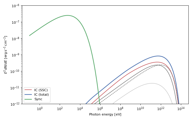
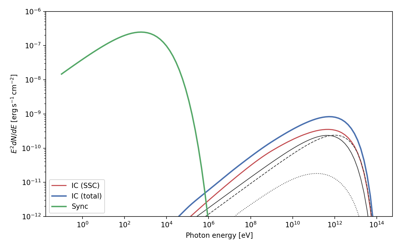
Note the factor 2.24 in the computation of the synchrotron photon density, which comes from geometrical considerations of a uniform spherical emitter (see Section 4.1 of Atoyan & Aharonian 1996). The resulting emission from Synchrotron and Inverse Compton can then be plotted:

(Source code, png, hires.png, pdf)

One of the only galactic sources where SSC is a relevant emission channel at gamma-rays is the Crab Nebula. With naima we can attempt a simple model to explain most of its non-thermal features. Assuming a present-age electron spectrum with an energy distribution described by a broken power law with indices 1.5 and 3.2, and an exponential cutoff at 1.8 PeV, a uniform magnetic field strenght of 125 \(\mu G\), and a size of 2.1 pc, we obtain the following SED (the full script to generate this model can be found in the examples page Crab Nebula SSC model):

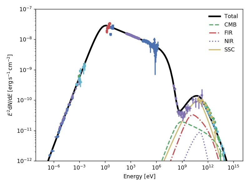
Note that this is a very crude representation of the physics of the Crab Nebula, and as a result some of the features are not well represented, most notably the flux at GeV energies. The reason is likely the simplification of the electron distribution into a broken power law rather than two components: a relic electron population emitting mostly at radio, and a high-energy wind electron population (see, e.g. Atoyan & Aharonian (1996) or Meyer et al. (2010)).

Synchrotron

Synchrotron radiation is produced by all charged particles in the presence of magnetic fields, and is ubiquitous in the emitted spectrum of leptonic sources. A full description and derivation of its properties can be found in Blumenthal & Gould (1970). The derivation of the spectrum is usually done considering a uniform magnetic field direction, but that is rarely thought to be the case in astrophysical sources. Considering random magnetic fields results in a shift of the maximum emissivity from \(E_\mathrm{peak}=0.29 E_\mathrm{c}\) to \(0.23 E_c\), where \(E_c\) is the synchrotron characteristic energy. The Synchrotron class implements the parametrization of the emissivity function of synchrotron radiation in random magnetic fields presented by Aharonian et al. (2010; Appendix D). This parametrization is particularly useful as it avoids using special functions, and achieves an accuracy of 0.2% over the entire range of emission energy.

To acknowledge the use of this implementation in your research, please cite Aharonian, F.A., Kelner, S.R., & Prosekin, A.Y. 2010, Physical Review D, 82, 043002.

Nonthermal Bremsstrahlung

Nonthermal bremsstrahlung radiation arises when a population of relativistic particles interact with a thermal particle population (see Blumenthal & Gould 1970). For the computation of the bremsstrahlung emission spectrum, The Bremsstrahlung class implements the approximation of Baring et al. (1999) to the original cross-section presented by Haug (1975). Electron-electron bremsstrahlung is implemented for the complete energy range, whereas electron-ion bremsstrahlung is at the moment only available for photon energies above 10 MeV. The normalization of the emission, and importance of the electron-electron versus the electron-ion channels, are given by the class arguments n0 (ion total number density), weight_ee (weight of the e-e channel, given by \(\sum_i Z_i X_i\)), and weight_ep (weight of the e-p channel, given by \(\sum_i Z_i^2 X_i\)). The defaults for weight_ee and weight_ep correspond to a fully ionised medium with solar abundances.

To acknowledge the use of this implementation in your research, please cite Baring, M.G., Ellison, D.C., Reynolds, S.P., Grenier, I.A., & Goret, P. 1999, Astrophysical Journal, 513, 311.

Pion Decay

The main gamma-ray production for relativistic protons are p-p interactions followed by pion decay, which results in a photon with \(E_\gamma > 100\,\mathrm{MeV}\). Until recently, the only parametrizations available for the integral cross-section and photon emission spectra were either only applicable to limited energy ranges, or were given as extensive numerical tables (e.g., Kelner et al. 2006; Kamae et al. 2006). By considering Monte Carlo results and a compilation of accelerator data on p-p interactions, Kafexhiu et al. (2014) were able to develop analytic parametrizations to the energy spectra and production rates of gamma rays from p-p interactions. The PionDecay class uses an implementation of the formulae presented in their paper, and gives the choice of which high-energy model to use (from the parametrization to the different Monte Carlo results) through the hiEmodel parameter.

To acknowledge the use of this implementation in your research, please cite Kafexhiu, E., Aharonian, F., Taylor, A.M., & Vila, G.S. 2014, Physical Review D, 90, 123014.